Taking Advantage of Custom Arrays in Google Sheets

[randy]

One feature in Google Sheets that I find incredibly helpful that isn’t well understood is the ability to build custom arrays/ranges within formulas. The Google Sheets documentation has a brief & unassuming callout to this capability that does not really acknowledge its power or potential.

Let’s dig into how this capability works and how to use it to super charge your spreadsheets…

Building Custom Ranges

The documentation above shows some pretty simple examples.

Fundamentals

In essence, you can use brackets { } to create multi-cell ranges.

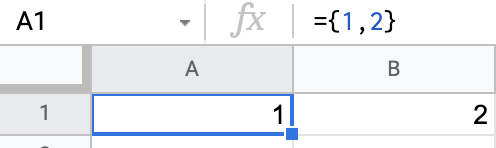
Separating values with commas (e.g. ={ 1 , 2 } creates an array with columns.

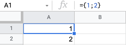
Separating values with semicolons (e.g. ={ 1 ; 2 } creates an array with rows.

These two concepts can be combined to create two-dimensional arrays-within-arrays (e.g. ={ { 1, 2 } ; { 3 , 4 } } creates an array with rows.

Arrays of Ranges

While it is sometimes helpful to create static custom arrays as in the examples above , this capability becomes more powerful when used to stitch together cell ranges in your sheets into custom arrays.

For example, using the formula ={A1:A3,C1:C3}, you can see that our custom array pulls just the first and third columns from the three columns of data above it (it skips the middle column, column B).

Applications

So now that we understand how to build custom arrays, how can we use them to improve our spreadsheets? Below, I’ve provided a few examples of the ways I often use them.

Single-cell Header + Formula Rows

When possible, I try to embedded key column-spanning formulas in my header rows. This approach allows users to add and delete rows in the table body without disrupting the formulas.

Let’s understand how this formula works:
={"Double Value";ARRAYFORMULA(2*A2:A)}

You can see that we create a custom array with the first row being the static text "Double Value". After that, a semicolon separates data vertically (i.e. new row) and below that we use an ARRAYFORMULA() to dynamically calculate allow content below the header as the data in column A but multiplied by 2.

This multiply-by-two formula is simple, but you can create much more elaborate formulas with this approach that included nested if-statements and VLOOKUPS(). For example, the output can been made more pretty and performant like this:
={"Double Value";ARRAYFORMULA(IF(ISBLANK(A2:A),IFERROR(1/0),2*A2:A))}

Less Brittle VLOOKUP()

The VLOOKUP() function can be a powerful way to find linked data from other sources but, because of the third parameter which identifies the column index, it can be brittle when a user adds or removes columns within its search range. Let’s look at this basic example:
=VLOOKUP(C2,A2:B,2,FALSE)

If the user were to add a Middle Name column between columns A and B, you can imagine that the direct reference to the range in the VLOOKUP() would expand from A2:B to A2:C. But Sheets isn’t smart enough to update the static number 2 for the column index. So, essentially, if we added this middle-name column, the VLOOKUP() would change to lookup the middle name from the first name provided in column C (D after the imaginary column insertion if you are spatially intuitive and following along closely ).

The solution to this problem is to build your VLOOKUP() range from a custom array in this way:
=VLOOKUP(C2,{A2:A,B2:B},2,FALSE)

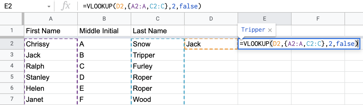
In this approach, rather than providing a block range, we pull in just the columns that are needed for our lookup. The search column is always first. The result column is always second. So the static column index (2) remains unchanged. If the user were to add a Middle Name column between columns A and B, you can imagine that the direct references would update as follows (and that the lookup would still correctly find the last name value):
=VLOOKUP(D2,{A2:A,C2:C},2,FALSE)

Reverse VLOOKUP()

Have you ever noticed that the search/lookup column in a VLOOKUP() formula must always be the first? What if you want to find data using a column in the middle of your range and return a value from a column to the left of that? The solution is pretty straightforward using the approach above.

Using the following formula, we can use a last name to lookup a first name:
=VLOOKUP(D2,{C2:C,A2:A},2,FALSE)

P.S. I learned this trick from Ben Collins long ago.

Dynamic Data Ranges with ARRAYFORMULA()

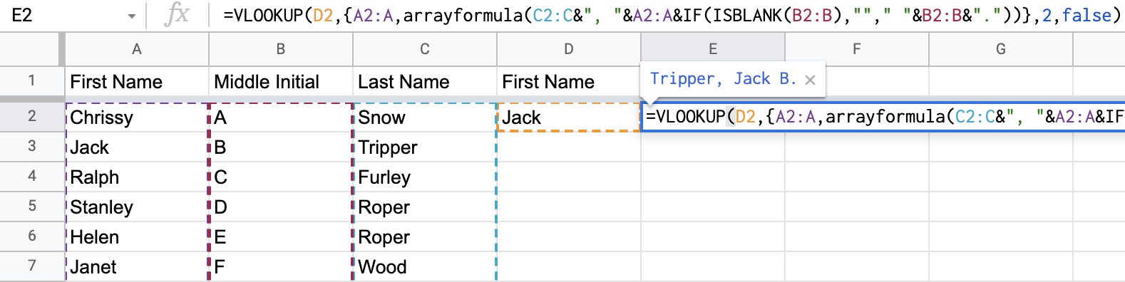
Another cool usage of custom ranges is the capability to dynamically generate derived data and to include that virtual, formula-created array as a range. In the example below, our VLOOKUP() function searches for the first name in D2 in the first-column range (A2:A) but the returned value is a dynamically-generated full name column created within the formula using ARRAYFORMULA():
=VLOOKUP(D2,{A2:A,ARRAYFORMULA(C2:C&", "&A2:A&IF(ISBLANK(B2:B),""," "&B2:B&"."))},2,FALSE)

This approach works great with VLOOKUP() but dynamically-generated data ranges can be used as source ranges for all sorts of functions including QUERY() .

Custom QUERY() Ranges

Similar to the "Less Brittle VLOOKUP()" example, the QUERY() function can be easily compromised by the addition or removal of columns in its range parameter. Let’s take a look at this example:
=QUERY(A2:C7,"SELECT C, A ORDER BY C, A LIMIT 4")

Here, we are using the QUERY() function to return the first 4 last- then first-names in alphabetical order. We are referencing columns by their letters (e.g. C and A) in the provided range.

As with the brittle VLOOKUP() example, if a user deleted middle-initial column B, you can imagine that the direct reference in the formula would update to:
=QUERY(A2:B7,"SELECT C, A ORDER BY C, A LIMIT 4")

The problem is that Sheets isn’t quite smart enough to update the static query text, so the query will try to select data from column C which is outside of the (new) range and will crash the query.

What is the solution? You’re getting the hang of this, right? It’s to package our data ranges within a custom array like this (we can skip over the middle-initial column since our query doesn’t use it):
=QUERY({A2:A7,C2:C7},"SELECT Col2, Col1 ORDER BY Col2, Col1 LIMIT 4")

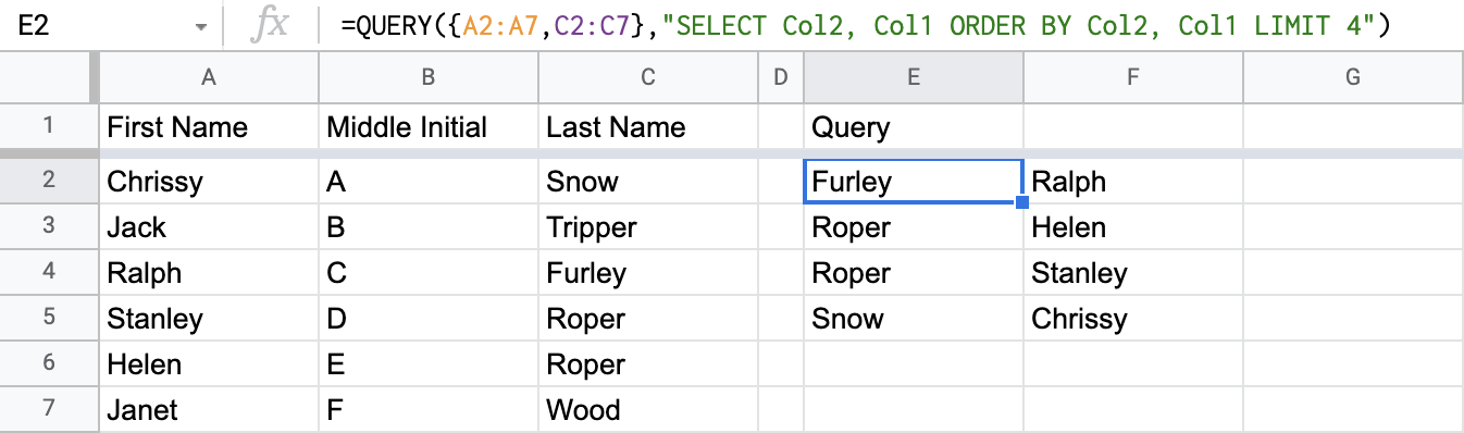
An important note here is that we cannot reference columns using their Sheets column letters if our data is not provided from a cell range. You can see in the formula above, we reference column C using Col2 based on the provided column order in the custom array and column A is referenced using Col1.

[Cowboy13]

Randy,
Very useful information on a powerful feature that seems to have scarce documentation. The reverse VLookup is something I just recently discovered by experimentation and was pleasantly surprised it worked!

Thanks.

[dyoung418]

Another solution for QUERY that I frequently use is to build in MATCH expressions into the query to match by column header.
In your example, the solution would look like this:

=QUERY({A2:C7}, "SELECT Col"&MATCH("Last Name",A2:C2,0)& 
", Col"&MATCH("First Name",A2:C2,0)&
" ORDER BY Col"&MATCH("Last Name",A2:C2,0)&
", Col"&MATCH("First Name",A2:C2,0)&
" LIMIT 4")

Messy to read until you get used to it, but very robust in the face of columns moving around, or accidentally specifying the wrong column initially.

[morgan]

@dyoung418 Thanks for sharing!

[randy]

That’s interesting, @dyoung418. I hadn’t thought of that.

[diogo6]

This is very cool indeed! I use a similar notion often on my base g-sheets scripts but, again, this can be quite helpful, and I hope I remember to use it soon enough. Bravo.

[ScottC]

As @dyoug418 says, this formula is messy to read. I’m not an advanced Sheets but I’m constantly impressed by its power and that by those that know how to use it. When I see formulas like this I ask one of the AI’s to explain it. Their explanations are always surprisingly clear. This is how ChatGPT v4 explains @dyoung481’s Query formula:

This Google Sheets formula is using the QUERY function to select and order data from a range (in this case, A2:C7). Let’s break it down step-by-step:

1. QUERY function: The QUERY function in Google Sheets allows you to run a SQL-like query on your data. The general syntax is:
   [
   \text{QUERY(data, query_string, [headers])}
   ]
   where:

   • data is the range of data you want to query.
   • query_string is the actual SQL-like query you want to run on the data.
   • [headers] is an optional argument specifying how many rows to treat as headers.

2. Array Notation {A2:C7}: The curly braces {} are used to denote an array. In this formula, it simply refers to the range A2:C7.

3. MATCH function: The MATCH function searches for a value (in this case, a string like “Last Name” or “First Name”) in a range and returns the relative position of that item. The syntax for the MATCH function is:
   [
   \text{MATCH(search_key, range, [search_type])}
   ]
   where:

   • search_key is the value you’re looking for.
   • range is the range where you want to search.
   • [search_type] is an optional argument, which in this formula is set to 0, meaning an exact match.

4. Putting it all together:

   • "SELECT Col"&MATCH("Last Name",A2:C2,0)& ", Col"&MATCH("First Name",A2:C2,0): This part constructs the SELECT clause of the query. It selects the columns corresponding to “Last Name” and “First Name” based on their positions in the range A2:C2.

   • " ORDER BY Col"&MATCH("Last Name",A2:C2,0)& ", Col"&MATCH("First Name",A2:C2,0): This part constructs the ORDER BY clause of the query. It orders the results first by “Last Name” and then by “First Name” based on their positions.

   • " LIMIT 4": This limits the results to the first 4 rows.

So, in essence, the formula is querying the range A2:C7, selecting the columns corresponding to “Last Name” and “First Name”, ordering the results by “Last Name” and then “First Name”, and finally limiting the output to the first 4 rows.

[dyoung418]

Wow, that’s an impressive explanation by ChatGPT, and spot on!

[ppraju12]

Thanks for sharing this @randy!!
The Reverse VLOOKUP and Custom Query Ranges seems pretty useful.

These are pretty nifty ways to combine arrays of ranges, queries and VLOOKUP together.

[rhowell]

I spent a lot of time looking for ways to make QUERY more dynamic. (Wouldn’t it be great if it lived up to its documentation and accepted header names as references?)

An alternative to the MATCH solution proposed by @dyoung418 can be found here: google sheets - Can I use column headers in a =QUERY? - Web Applications Stack Exchange

It uses a lambda function to parse header name input into Col1-type references. I think it does a nice job of preserving readability while reducing brittleness. (Note that it doesn’t handle special characters in header names very well.)

I rewrote it to be a bit clearer about the name arguments (this example will pull your latest balances for asset accounts):

 =LAMBDA(data_, query_, headers_,
    QUERY({data_}, 
      LAMBDA(query_text_, data_row1_,
        REDUCE(query_text_, FILTER(data_row1_, ISTEXT(data_row1_)), 
          LAMBDA(query_text_result_, data_col_name_, REGEXREPLACE(query_text_result_, "`" & data_col_name_ & "`", "Col" & MATCH(data_col_name_, data_row1_, 0)))))
      (query_, ARRAY_CONSTRAIN(data_, 1, COLUMNS(data_))), 
    headers_))
(Accounts!G:ZZ, "select `Account`, `Last Update`, `Last Balance` where `Account` is not null and `Class` = 'Asset' and `Hide` <> 'Hide'", 1)

[dyoung418]

I love this! This will be my new way of going about queries. The full formula looks complex, but you can ignore all of it except the last line, which is very easy to read; and if you implement the Named Function for the LAMBDA as the original poster suggests, it is the solution that I have wished QUERY had implemented all along. Thanks for posting this @rhowell !

[randy]

That’s a cool use of a LAMBDA function, @rhowell. Hadn’t seen this approach. Thanks for sharing.

[Mark.S]

That is pretty slick!

The Accounts sheet is a small dataset, but I was curious - if QUERY is run using a large dataset (like the Transactions sheet A:ZZ), is there a performance tradeoff vs. a custom array of only the needed data?

Does QUERY load the entire dataset into memory, even though say only 2 or 3 columns are used?

[rhowell]

I’ve been using this lambda-query pretty indiscriminately to pull data from my 8,000+ transactions (Transactions!A:ZZ) and haven’t noticed any performance problems. I’ve even been tacking additional arrays (of, e.g., category groups via an xlookup) onto the full Transactions array.

However, it seems that the more you do before writing to cells, the better: If I lamba-query and select * with no where constraints, the sheet slows considerably. If I perform the same query but then further refine the data (via additional queries, filters, etc.) in the same formula, no problems.