Hello everyone, have you heard of a pivot table? In short a pivot table summarizes data. You can create one in either Google Sheets or Excel, although they have different interfaces.
Why Use a Pivot Table with Your Tiller Data?
The Tiller Community is home to so many powerful, prebuilt templates for budgeting, tracking net worth, and managing debt. They are fantastic for structured analysis over the long term.
But sometimes, you just have a quick, specific question you want to answer immediately, without building a whole new sheet or writing complex formulas. This is where a pivot table is your best friend.
A pivot table is the perfect tool when you want to:
- Get instant answers: Find out “How much did I spend at Amazon last quarter?” or “What were my top 5 spending categories in June?” in seconds.
- Analyze trends without formulas: Instead of writing complicated SUMIFS or VLOOKUP functions, you can just drag and drop to see your spending by month, by quarter, or by year.
- Explore your data: Quickly group all your transactions by Merchant to see where your money really goes, or group by Category to see your totals.
- Be flexible: A template is built for a specific purpose. A pivot table lets you change your mind. You can “pivot” your data instantly, swap rows and columns, add a filter for “Groceries,” or remove a “Transfer” category, all on the fly.
- Verify your budget: Use a pivot table to quickly sum up your Transactions sheet and apply a filter for your tags if you use them.
How to Make a Pivot Table in Google Sheets
-
First, go to your Transactions sheet.
-
Highlight the columns.
-
From the top menu, click Insert, and then find Pivot table.
-
A small box will pop up. It will ask where to put it. Always choose New sheet. This keeps your Transactions sheet clean. Click Create.
-
You’ll see a blank table and a Pivot table editor on the right side. This editor is your control panel. It has four boxes: Rows, Columns, Values, and Filters.
-
Start with ROWS. This is, confusingly, the column that you want to summarize. If you keep the description uniform, this can be a good choice to see how much you spend on each merchant. I have set up an advanced AutoCat rule to change all of the “McDonalds…” that have the store number or sometimes use an apostrophe, into a uniform “McDonalds” so I can see how much I spend there, even if I went to different stores.
-
Skip the Columns option for now. That is how you can split the rows into subcategories. When I was a math teacher I used Columns to split quiz questions by class period: 1st period, 2nd period, etc… If you have a tags column it might be helpful to utilize the “Columns” option in the pivot table editor.
-
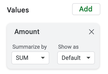
Values is what column you are summarizing. Probably you want the Amount column.
The default “Summarize by” is Sum, which adds up all of the values per merchant, in this example. You may want to change that to COUNT or COUNTA to see how many times you went to McDonalds. -
Filter is where the pivot table really shines. You can filter by date, tag, merchant, etc…
Choose the column you want to filter by, for example date. Click on the dropdown for “Showing all items.” Click on “Clear” to deselect all items, then you can click to select the ones you do want.
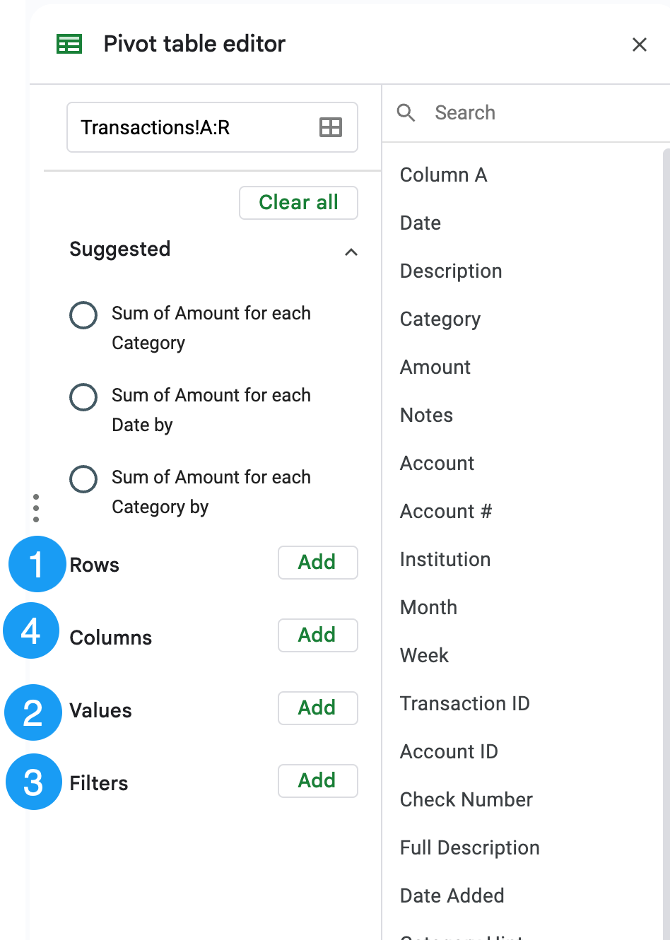

Note: You can also filter by condition, to have dates after a certain period for example.
How to Make a PivotTable in Excel
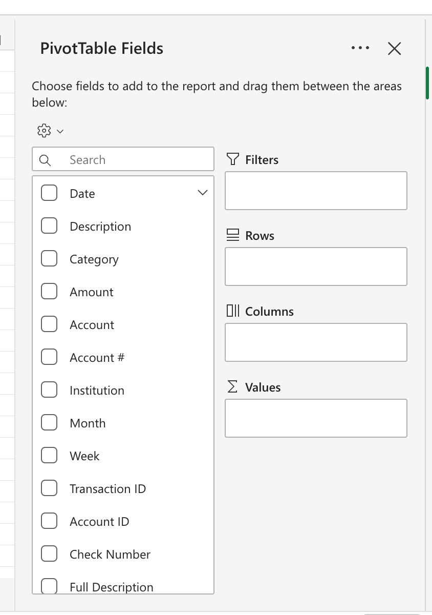
The steps in Excel are almost identical. The main difference is that Excel calls its editor “PivotTable Fields”.

- Open your Transactions sheet.
- Highlight the columns.
- Go to the Insert tab on the top ribbon and click the PivotTable button.
- A sidebar will appear. It will suggest pivot tables to you, of course you are free to use one of those. Otherwise, at the top choose the option to create a pivot table in a new sheet.
- You now have a blank table on the left and your control panel, the PivotTable Fields pane, on the right. The order of the 4 fields are different: Filters, Rows, Columns, Values.
- DRAG the fields into each of the boxes. Notice that when you drag Amount into the Values box, it says “Sum of Amount” and it is a dropdown. You can change this to summarize with counting or the maximum value if you want.
What pivot table tips do you have?
-Alice
Tiller Evangelist