Overview (Updated to 2.1 in March 2026- new features)
Now that I have multiple years of transactions in my Tiller sheet, I want to be able to see my annual Income and Expenses for multiple years on one page and wanted to know what my average was over the number of years I choose.
In addition, I wanted to see, by Category and Category Group, my annual Income and Expenses over a period of years without certain Categories or Category Groups. One reason why? I am getting closer to retirement and want to know what spending has been without expenses that will be gone by retirement- e.g. kids college expenses, loan payments that will be paid off, getting rid of a car, etc.
I thought this would have existed but couldn’t find it so I created my own. I actually started with another worksheet I had already modified a while ago because I liked the layout. However, It’s been so long, I don’t remember the original source of the worksheet so I apologize to the original author!

Installation
You can download the worksheet from here…
Copy the worksheet into your Tiller workbook and you’re good to go. It uses the Transaction and Category worksheets.
Setup
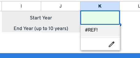
To setup, the only thing you have to do is choose the Start and End year…

Once you pick the starting year, it will only allow up to 10 years to pull. This is simply a limitation I put in to limit the number of columns to display. Also, the earliest year it will allow you to use is the first year you have a transaction.
You also have show and sort options (new for 2.0)…

You can show- Groups and Categories, Groups only, or Categories only. You can sort on Item (Groups and Categories) or Total $s, ascending or descending.
You can also choose to exclude Categories or Category Groups from the table so you can see the totals with these items.
To do this, hit the “+” above column R to display the following columns…

There is no limit to the number of Groups and Categories you can exclude (new for 2.0).
For example, here are my Auto Expenses, including insurance for my daughter’s Kia Soul…

I then choose to exclude this Category…
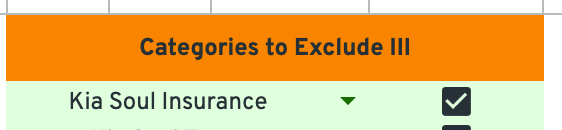
and it no longer shows up in the data…

Permissions
I encourage others to copy, use, and modify however you want.
Notes
-
It will not display any Categories or Category Groups that have $0 for the years you choose
-
In columns T and U, you can also choose to Show Hidden Categories or Transfers or blank rows between Groups…
-
I purposely kept this very simple- no charts, no limiting by accounts, etc. However, with a few tweaks all of these items are possible. However, I don’t see the benefit for my use.
-
For the Average, it will calculate a simple average over the years you choose. If the final year you choose is the current year, current year totals = actuals through completed months + remaining budget for the year.
-
In 2.1, I optimized the formulas, corrected some minor bugs, and added additional features.
-
It will produce bad data for any of your Types, Groups, and Categories that have the same name. For example, if you have a Group named “Auto” and a Category also named “Auto”, the data for that name will be incorrect. Make sure the names are not repeated.

Would love to hear your comments, feedback, suggestions for improvements, or questions.
Enjoy.